Working with Streaming Data

import time

import numpy as np
import pandas as pd

import holoviews as hv
from holoviews import opts
from holoviews.streams import Buffer, Pipe

hv.extension('bokeh')

Pipe

A Pipe allows data to be pushed into a DynamicMap callback to change a visualization, just like the streams in the Responding to Events user guide were used to push changes to metadata that controlled the visualization. A Pipe can be used to push data of any type and make it available to a DynamicMap callback. Since all Element types accept data of various forms we can use Pipe to push data directly to the constructor of an Element through a DynamicMap.

We can take advantage of the fact that most Elements can be instantiated without providing any data, so we declare the the Pipe with an empty list, declare the DynamicMap, providing the pipe as a stream, which will dynamically update a VectorField :

pipe = Pipe(data=[])
vector_dmap = hv.DynamicMap(hv.VectorField, streams=[pipe])
vector_dmap.opts(color='Magnitude', xlim=(-1, 1), ylim=(-1, 1))

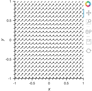
Having set up this VectorField tied to a Pipe we can start pushing data to it varying the orientation of the VectorField:

x,y  = np.mgrid[-10:11,-10:11] * 0.1
sine_rings  = np.sin(x**2+y**2)*np.pi+np.pi
exp_falloff = 1/np.exp((x**2+y**2)/8)

for i in np.linspace(0, 1, 25):
    time.sleep(0.1)
    pipe.send((x,y,sine_rings*i, exp_falloff))

This approach of using an element constructor directly does not allow you to use anything other than the default key and value dimensions. One simple workaround for this limitation is to use functools.partial as demonstrated in the Controlling the length section below.

Since Pipe is completely general and the data can be any custom type, it provides a completely general mechanism to stream structured or unstructured data. Due to this generality, Pipe does not offer some of the more complex features and optimizations available when using the Buffer stream described in the next section.

Buffer

While Pipe provides a general solution for piping arbitrary data to DynamicMap callback, Buffer on the other hand provides a very powerful means of working with streaming tabular data, defined as pandas dataframes, arrays or dictionaries of columns (as well as StreamingDataFrame, which we will cover later). Buffer automatically accumulates the last N rows of the tabular data, where N is defined by the length.

The ability to accumulate data allows performing operations on a recent history of data, while plotting backends (such as bokeh) can optimize plot updates by sending just the latest patch. This optimization works only if the data object held by the Buffer is identical to the plotted Element data, otherwise all the data will be updated as normal.

A simple example: Brownian motion

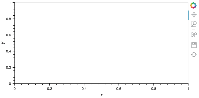
To initialize a Buffer we have to provide an example dataset which defines the columns and dtypes of the data we will be streaming. Next we define the length to keep the last 100 rows of data. If the data is a DataFrame we can specify whether we will also want to use the DataFrame index. In this case we will simply define that we want to plot a DataFrame of ‘x’ and ‘y’ positions and a ‘count’ as Points and Curve elements:

example = pd.DataFrame({'x': [], 'y': [], 'count': []}, columns=['x', 'y', 'count'])
dfstream = Buffer(example, length=100, index=False)
curve_dmap = hv.DynamicMap(hv.Curve, streams=[dfstream])
point_dmap = hv.DynamicMap(hv.Points, streams=[dfstream])

After applying some styling we will display an Overlay of the dynamic Curve and Points

(curve_dmap * point_dmap).opts(
    opts.Points(color='count', line_color='black', size=5, padding=0.1, xaxis=None, yaxis=None),
    opts.Curve(line_width=1, color='black'))

Now that we have set up the Buffer and defined a DynamicMap to plot the data we can start pushing data to it. We will define a simple function which simulates brownian motion by accumulating x, y positions. We can send data through the hv.streams.Buffer directly.

def gen_brownian():
    x, y, count = 0, 0, 0
    while True:
        x += np.random.randn()
        y += np.random.randn()
        count += 1
        yield pd.DataFrame([(x, y, count)], columns=['x', 'y', 'count'])

brownian = gen_brownian()
for _ in range(200):
    dfstream.send(next(brownian))

Finally we can clear the data on the stream and plot using the clear method:

dfstream.clear()

Note that when using the Buffer stream the view will always follow the current range of the data by default, by setting buffer.following=False or passing following as an argument to the constructor this behavior may be disabled.

Asynchronous updates using asyncio

In most cases, instead of pushing updates manually from the same Python process, you’ll want the object to update asynchronously as new data arrives. Since both Jupyter and Bokeh server run on an asyncio event-loop in both cases to define a non-blocking co-routine that can push data to our stream whenever it is ready. We can define an asynchronous functionwith a asyncio.sleep timeout and schedule it as a task. Once we have declared the callback we can call start to begin emitting events:

import asyncio

count = 0
buffer = Buffer(np.zeros((0, 2)), length=50)

async def f():
    global count
    while True:
        await asyncio.sleep(0.1)
        count += 1
        buffer.send(np.array([[count, np.random.rand()]]))

task = asyncio.create_task(f())

hv.DynamicMap(hv.Curve, streams=[buffer]).opts(padding=0.1, width=600)

Since the callback is non-blocking we can continue working in the notebook and execute other cells. Once we’re done we can stop the callback by calling cb.stop().

task.cancel()

Real examples

Using the Pipe and Buffer streams we can create complex streaming plots very easily. In addition to the toy examples we presented in this guide it is worth looking at looking at some of the examples using real, live, streaming data.

• The streaming_psutil bokeh app is one such example which display CPU and memory information using the psutil library (install with pip install psutil or conda install psutil)

As you can see, streaming data works like streams in HoloViews in general, flexibly handling changes over time under either explicit control or governed by some external data source.

This web page was generated from a Jupyter notebook and not all interactivity will work on this website. Right click to download and run locally for full Python-backed interactivity.